$$ \newcommand{\defeq}{\stackrel{\small\bullet}{=}} \newcommand{\ra}{\rangle} \newcommand{\la}{\langle} \newcommand{\norm}[1]{\left\|#1\right\|} \newcommand{\abs}[1]{\left\lvert#1\right\rvert} \newcommand{\Abs}[1]{\Bigl\lvert#1\Bigr\rvert} \newcommand{\pr}{{\mathbb P}} \newcommand{\qr}{{\mathbb Q}} \newcommand{\xv}{{\boldsymbol{x}}} \newcommand{\av}{{\boldsymbol{a}}} \newcommand{\bv}{{\boldsymbol{b}}} \newcommand{\cv}{{\boldsymbol{c}}} \newcommand{\dv}{{\boldsymbol{d}}} \newcommand{\ev}{{\boldsymbol{e}}} \newcommand{\fv}{{\boldsymbol{f}}} \newcommand{\gv}{{\boldsymbol{g}}} \newcommand{\hv}{{\boldsymbol{h}}} \newcommand{\nv}{{\boldsymbol{n}}} \newcommand{\sv}{{\boldsymbol{s}}} \newcommand{\tv}{{\boldsymbol{t}}} \newcommand{\uv}{{\boldsymbol{u}}} \newcommand{\vv}{{\boldsymbol{v}}} \newcommand{\wv}{{\boldsymbol{w}}} \newcommand{\zerov}{{\mathbf{0}}} \newcommand{\onev}{{\mathbf{0}}} \newcommand{\phiv}{{\boldsymbol{\phi}}} \newcommand{\cc}{{\check{C}}} \newcommand{\xv}{{\boldsymbol{x}}} \newcommand{\Xv}{{\boldsymbol{X}\!}} \newcommand{\yv}{{\boldsymbol{y}}} \newcommand{\Yv}{{\boldsymbol{Y}}} \newcommand{\zv}{{\boldsymbol{z}}} \newcommand{\Zv}{{\boldsymbol{Z}}} \newcommand{\Iv}{{\boldsymbol{I}}} \newcommand{\Jv}{{\boldsymbol{J}}} \newcommand{\Cv}{{\boldsymbol{C}}} \newcommand{\Ev}{{\boldsymbol{E}}} \newcommand{\Fv}{{\boldsymbol{F}}} \newcommand{\Gv}{{\boldsymbol{G}}} \newcommand{\Hv}{{\boldsymbol{H}}} \newcommand{\alphav}{{\boldsymbol{\alpha}}} \newcommand{\epsilonv}{{\boldsymbol{\epsilon}}} \newcommand{\betav}{{\boldsymbol{\beta}}} \newcommand{\deltav}{{\boldsymbol{\delta}}} \newcommand{\gammav}{{\boldsymbol{\gamma}}} \newcommand{\etav}{{\boldsymbol{\eta}}} \newcommand{\piv}{{\boldsymbol{\pi}}} \newcommand{\thetav}{{\boldsymbol{\theta}}} \newcommand{\tauv}{{\boldsymbol{\tau}}} \newcommand{\muv}{{\boldsymbol{\mu}}} \newcommand{\phiinv}{\Phi^{-1}} \newcommand{\Fiinv}{F^{-1}} \newcommand{\giinv}{g^{-1}} \newcommand{\fhat}{\hat{f}} \newcommand{\ghat}{\hat{g}} \newcommand{\ftheta}{f_\theta} \newcommand{\fthetav}{f_{\thetav}} \newcommand{\gtheta}{g_\theta} \newcommand{\gthetav}{g_{\thetav}} \newcommand{\ztheta}{Z_\theta} \newcommand{\xtheta}{\Xv_\theta} \newcommand{\ytheta}{\Yv_\theta} \newcommand{\p}{\partial} \newcommand{\f}{\frac} \newcommand{\cf}{\cfrac} \newcommand{\e}{\epsilon} \newcommand{\indep}{\perp\kern-5pt \perp} \newcommand{\inner}[1]{\langle#1\rangle} \newcommand{\pa}[1]{\left(#1\right)} \newcommand{\pb}[1]{\left\{#1\right\}} \newcommand{\pc}[1]{\left[#1\right]} \newcommand{\pA}[1]{\Big(#1\Big)} \newcommand{\pB}[1]{\Big\{#1\Big\}} \newcommand{\pC}[1]{\Big[#1\Big]} \newcommand{\ty}[1]{\texttt{#1}} \newcommand{\borel}[1]{\mathscr{B}\pa{#1}} \newcommand{\scr}{\mathcal} \newcommand{\scrb}{\mathscr} \newcommand{\argmin}{\mathop{\text{arg}\ \!\text{min}}} \newcommand{\arginf}{\mathop{\text{arg}\ \!\text{inf}}} \newcommand{\argmax}{\mathop{\text{arg}\ \!\text{max}}} \newcommand{\argsup}{\mathop{\text{arg}\ \!\text{sup}}} \newcommand{\bigo}[1]{\mathcal{O}_{p}\!\left(#1\right)} \newcommand{\f}{\frac} \newcommand{\e}{\epsilon} \newcommand{\inv}{^{-1}} \newcommand{\phiinv}{\Phi^{-1}} \newcommand{\Fiinv}{F^{-1}} \newcommand{\giinv}{g^{-1}} \newcommand{\fhat}{\hat{f}} \newcommand{\ghat}{\hat{g}} \newcommand{\ftheta}{f_\theta} \newcommand{\fthetav}{f_{\thetav}} \newcommand{\gtheta}{g_\theta} \newcommand{\gthetav}{g_{\thetav}} \newcommand{\ztheta}{Z_\theta} \newcommand{\xtheta}{\Xv_\theta} \newcommand{\ytheta}{\Yv_\theta} \newcommand{\absdet}[1]{\abs{\det\pa{#1}}} \newcommand{\jac}[1]{\Jv_{#1}} \newcommand{\absdetjx}[1]{\abs{\det\pa{\Jv_{#1}}}} \newcommand{\absdetj}[1]{\norm{\Jv_{#1}}} \newcommand{\sint}{sin(\theta)} \newcommand{\cost}{cos(\theta)} \newcommand{\sor}[1]{S\mathcal{O}(#1)} \newcommand{\ort}[1]{\mathcal{O}(#1)} \newcommand{\A}{{\mathcal A}} \newcommand{\C}{{\mathbb C}} \newcommand{\E}{{\mathbb E}} \newcommand{\F}{{\mathcal{F}}} \newcommand{\N}{{\mathbb N}} \newcommand{\R}{{\mathbb R}} \newcommand{\Q}{{\mathbb Q}} \newcommand{\Z}{{\mathbb Z}} \newcommand{\X}{{\mathbb{X}}} \newcommand{\Y}{{\mathbb{Y}}} \newcommand{\G}{{\mathcal{G}}} \newcommand{\M}{{\mathcal{M}}} \newcommand{\betaequivalent}{\beta\text{-equivalent}} \newcommand{\betaequivalence}{\beta\text{-equivalence}} \newcommand{\Mb}{{\boldsymbol{\mathsf{M}}}} \newcommand{\Br}{{\mathbf{\mathsf{Bar}}}} \newcommand{\dgm}{{\mathfrak{Dgm}}} \newcommand{\Db}{{\mathbf{\mathsf{D}}}} \newcommand{\Img}{{\mathbf{\mathsf{Img}}}} \newcommand{\mmd}{{\mathbf{\mathsf{MMD}}}} \newcommand{\Xn}{{\mathbb{X}_n}} \newcommand{\Xm}{{\mathbb{X}_m}} \newcommand{\Yn}{{\mathbb{Y}_n}} \newcommand{\Ym}{Y_1, Y_2, \cdots, Y_m} \newcommand{\Xb}{{\mathbb{X}}} \newcommand{\Yb}{{\mathbb{Y}}} \newcommand{\s}{{{\sigma}}} \newcommand{\fnsbar}{{\bar{f}^n_\s}} \newcommand{\fns}{{f^n_\s}} \newcommand{\fs}{{f_\s}} \newcommand{\fsbar}{{\bar{f}_\s}} \newcommand{\barfn}{{{f}^n_\sigma}} \newcommand{\barfnm}{{{f}^{n+m}_\sigma}} \newcommand{\barfo}{{{f}_\sigma}} \newcommand{\fn}{{f^n_{\rho,\sigma}}} \newcommand{\fnm}{{f^{n+m}_{\rho,\sigma}}} \newcommand{\fo}{{f_{\rho,\sigma}}} \newcommand{\K}{{{K_{\sigma}}}} \newcommand{\barpn}{{\bar{p}^n_\sigma}} \newcommand{\barpo}{{\bar{p}_\sigma}} \newcommand{\pn}{{p^n_\sigma}} \newcommand{\po}{{p_\sigma}} \newcommand{\J}{{\mathcal{J}}} \newcommand{\B}{{\mathcal{B}}} \newcommand{\pt}{{\tilde{\mathbb{P}}}} \newcommand{\Winf}{{W_{\infty}}} \newcommand{\winf}{{W_{\infty}}} \newcommand{\HH}{{{\scr{H}_{\sigma}}}} \newcommand{\D}{{{\scr{D}_{\sigma}}}} \newcommand{\Ts}{{T_{\sigma}}} \newcommand{\Phis}{{\Phi_{\sigma}}} \newcommand{\nus}{{\nu_{\sigma}}} \newcommand{\Qs}{{\mathcal{Q}_{\sigma}}} \newcommand{\ws}{{w_{\sigma}}} \newcommand{\vs}{{v_{\sigma}}} \newcommand{\ds}{{\delta_{\sigma}}} \newcommand{\fp}{{f_{\pr}}} \newcommand{\prs}{{\widetilde{\pr}_{\sigma}}} \newcommand{\qrs}{{\widetilde{\qr}_{\sigma}}} \newcommand{\Inner}[1]{\Bigl\langle#1\Bigr\rangle} \newcommand{\innerh}[1]{\langle#1\rangle_{\HH}} \newcommand{\Innerh}[1]{\Bigl\langle#1\Bigr\rangle_{\HH}} \newcommand{\normh}[1]{\norm{#1}_{\HH}} \newcommand{\norminf}[1]{\norm{#1}_{\infty}} \newcommand{\gdelta}{{\G_{\delta}}} \newcommand{\supgdelta}{{\sup\limits_{g\in\gdelta}\abs{\Delta_n(g)}}} \newcommand{\id}{\text{id}} \newcommand{\supp}{\text{supp}} \newcommand{\cech}{\v{C}ech} \newcommand{\Zz}{{\scr{Z}}} \newcommand{\psis}{\psi_\s} \newcommand{\phigox}{\Phis(\xv)-g} \newcommand{\phigoy}{\Phis(\yv)-g} \newcommand{\fox}{{f^{\epsilon,{\xv}}_{\rho,\sigma}}} \newcommand{\prx}{{\pr^{\epsilon}_{\xv}}} \newcommand{\pro}{{\pr_0}} \newcommand{\dotfo}{\dot{f}_{\!\!\rho,\s}} \newcommand{\phifo}{{\Phis(\yv)-\fo}} \newcommand{\phifox}{{\Phis(\xv)-\fo}} \newcommand{\kinf}{{\norm{\K}_{\infty}}} \newcommand{\half}{{{\f{1}{2}}}} \newcommand{\Jx}{\J_{\epsilon,{\xv}}} \newcommand{\dpy}{\text{differential privacy}} \newcommand{\edpy}{$\epsilon$--\text{differential privacy}} \newcommand{\eedpy}{$\epsilon$--edge \text{differential privacy}} \newcommand{\dpe}{\text{differentially private}} \newcommand{\edpe}{$\epsilon$--\text{differentially private}} \newcommand{\eedpe}{$\epsilon$--edge \text{differentially private}} \newcommand{\er}{Erdős-Rényi} \newcommand{\krein}{Kreĭn} % \newcommand{\grdpg}{\mathsf{gRDPG}} % \newcommand{\rdpg}{\mathsf{RDPG}} % \newcommand{\eflip}{{\textsf{edgeFlip}}} % \newcommand{\grdpg}{\text{gRDPG}} % \newcommand{\rdpg}{\text{RDPG}} \newcommand{\grdpg}{\mathsf{gRDPG}} \newcommand{\rdpg}{\mathsf{RDPG}} \newcommand{\eflip}{{\text{edgeFlip}}} \newcommand{\I}{{\mathbb I}} \renewcommand{\pa}[1]{\left(#1\right)} \renewcommand{\pb}[1]{\left\{#1\right\}} \renewcommand{\pc}[1]{\left[#1\right]} \renewcommand{\V}{\mathbb{V}} \renewcommand{\W}{\mathbb{W}} %%%%%%%%%%%%%%%%%%%%%%%%%%% \providecommand{\fd}{\frac 1d} % \renewcommand{\fpp}{{\frac 1p}} \providecommand{\pfac}{\f{p}{p-1}} \providecommand{\ipfac}{\f{p-1}{p}} \providecommand{\dbq}{\Delta b_{n,m,Q}\qty(\qty{\xvo})} \providecommand{\db}{\Delta b_{n,m}\qty(\qty{\xvo})} \providecommand{\bbv}{{{\mathbb{V}}}} \providecommand{\bbw}{{{\mathbb{W}}}} \providecommand{\md}{\textsf{MoM Dist}} \providecommand{\bF}{{\mathbf{F}}} \providecommand{\sub}{{\text{Sub}}} \providecommand{\samp}{\text{$\pa{\scr{S}}$}} \providecommand{\tp}{{2^{\f{p-1}{p}}}} %%%%%%%%%%%%%%%%%%%%%%%%%% \providecommand{\Xmn}{{\mathbb{X}_{n+m}}} \newcommand{\Dnmq}{\D[n+m, Q]} \newcommand{\Dnmh}{\D[n+m, \H]} \newcommand{\Dn}{\D[n]} \providecommand{\xvo}{\xv_0} \providecommand{\bn}[1][\null]{b^{#1}_{n}\pa{\pb{\xvo}}} \providecommand{\bnm}[1][\null]{b^{#1}_{n+m}\pa{\pb{\xvo}}} \providecommand{\bnq}[1][\null]{b^{#1}_{n,Q}\pa{\pb{\xvo}}} \providecommand{\bnmq}[1][\null]{b^{#1}_{n+m,Q}\pa{\pb{\xvo}}}\providecommand{\prq}{\pr_q} \providecommand{\dxvo}{{\delta_{\xvo}}} \providecommand{\sq}{S_q} \providecommand{\Sq}{\abs{S_q}} \providecommand{\no}{{n_o}} \providecommand{\mmdn}{\mmd\pa{\pr_n, \delta_{\xvo}}} \newcommand{\rqt}{\xi_{q}(t; n, Q)} \providecommand{\nq}{\f{n}{Q}} \providecommand{\Ot}{\Omega(t, n/Q)} \providecommand{\ut}[1]{U^{#1}} \providecommand{\vt}[1]{V^{#1}} \providecommand{\wt}[1]{W^{#1}} \providecommand{\but}[1]{\mathbb{U}^{#1}} \providecommand{\bvt}[1]{\mathbb{V}^{#1}} \providecommand{\bwt}[1]{\mathbb{W}^{#1}} \providecommand{\ball}[1]{B_{f\!, \rho}\pa{#1}} \newcommand*{\medcap}{\mathbin{\scalebox{0.75}{{\bigcap}}}}% \newcommand*{\medcup}{\mathbin{\scalebox{0.75}{{\bigcup}}}}% \providecommand{\dsf}{\mathsf{d}} \newcommand{\Dnh}{{\mathsf{D}_{n,\scr{H}}}} \newcommand{\Dph}{{\mathsf{D}_{\pr,\scr{H}}}} \newcommand{\D}[1][1={ },usedefault]{{\mathsf{D}_{#1}}} \newcommand{\Dnq}{{\mathsf{D}_{n, Q}}} \newcommand{\dnq}{{\mathsf{d}_{n, Q}}} \newcommand{\dn}{{\mathsf{d}_{n}}} \newcommand{\dnm}{{\mathsf{d}_{n-m}}} \newcommand{\dmn}{{\mathsf{d}_{n+m}}} \newcommand{\dx}{{\mathsf{d}_{\mathbb{X}}}} \providecommand{\med}{\text{median}} \providecommand{\median}{\text{median}} \providecommand{\Xnm}{{\mathbb{X}^*_{n-m}}} $$

Week-1

Math 183 • Statistical Methods • Spring 2026

Siddharth Vishwanath

Learning objectives

Understanding data
Variable vs. Observation
Classification of Variables
Population Quantity vs. Sample Statistic
Implementation in R
Foundations of Data Summarization
Data Visualization Techniques

The Big Picture

Anatomy of Data

Sepal.Length	Sepal.Width	Petal.Length	Petal.Width	Species
5.1	3.5	1.4	0.2	setosa
4.9	3.0	1.4	0.2	setosa
4.7	3.2	1.3	0.2	setosa
4.6	3.1	1.5	0.2	setosa
5.0	3.6	1.4	0.2	setosa
5.4	3.9	1.7	0.4	setosa

Observation

An individual unit from which data are collected.

Anatomy of Data

Sepal.Length	Sepal.Width	Petal.Length	Petal.Width	Species
5.1	3.5	1.4	0.2	setosa
4.9	3.0	1.4	0.2	setosa
4.7	3.2	1.3	0.2	setosa
4.6	3.1	1.5	0.2	setosa
5.0	3.6	1.4	0.2	setosa
5.4	3.9	1.7	0.4	setosa

Variable

A characteristic for which different observations can take on different values.

Anatomy of Data

Observation

An individual unit from which data are collected.

Variable

A characteristic for which different observations can take on different values.

Constant

A characteristic that is the same for all observations

Coffee Consumption & Sleep Quality

A research team recruits 100 adults aged between 25-40 to participate in a 6-month study. Participants log their daily coffee intake and wear sleep trackers at night to record their sleep quality.

Observation: The adults
Variables: Coffee consumption frequency, Sleep quality
Constant: Age group (all adults are between 25-40)

Exercise Regime & Stress Levels

150 office workers are surveyed over a 3-month period where they report their weekly exercise routines and undergo monthly stress tests.

Observation: The individuals
Variables: Exercise regime, Stress levels
Constant: Time (all cases are measured in the same span of time)

Type of Cooking Oil & Heart Health

200 households in a city participate in a year-long study where their usage of cooking oil is recorded monthly. Additionally, all adult members undergo quarterly heart health check-ups.

Observation: The households
Variables: Type of cooking oil used, Heart health indicators
Constant: Geographic location (all households are in the same city)

Types of Variables

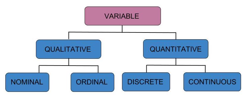
Warning

Sometimes computers can’t (or won’t) understand the difference between different types of variables. It’s up to us to tell them!

Examples

Beverage Preference

A survey in a school asks students their preferred beverage among tea, coffee, or juice.

Daily Screen Time

A study measures the daily screen time in hours of 100 individuals.

Types of Pets Owned

A neighborhood survey asks households about the types of pets they own.

Monthly Savings

Individuals are asked about their monthly savings in dollars.

Work Commute Method

A city survey asks residents about their preferred method of commuting to work.

Number of Books Read

A library conducts a survey asking individuals about the number of books they read in a month.

Favorite Music Genre

A radio station surveys its listeners to know their favorite music genre.

Weekly Exercise Hours

A health app collects data on the weekly exercise hours logged by its users.

Explanatory vs Response Variables

Explanatory Variable (Independent):
- The variable that is manipulated to observe its effects on another variable.
Response Variable (Dependent):
- The variable whose values are predicted or explained by the explanatory variable.

Example

A local gym aims to find the most effective workout routine for weight loss. They create a 3-month program where participants are divided into two groups. One group follows a cardio-centric routine, while the other engages in strength training. Participants’ weights are recorded at the start and end of the program. The gym seeks to understand which workout type leads to greater weight loss, to offer better guidance to its members.

Explanatory Variable: Type of exercise (e.g., cardio, strength training)
Response Variable: Amount of weight loss

Exercise Type & Weight Loss

A fitness center compares the effectiveness of two workout routines - HIIT and Yoga, for weight loss. The type of exercise is the explanatory variable, while the amount of weight loss is the response variable.

Teaching Methods & Student Performance

An educator evaluates two teaching methods to understand which one enhances student performance. The teaching method is the explanatory variable, and the students’ performance is the response variable.

Diet Type & Energy Levels

A nutritionist compares vegetarian and non-vegetarian diets to assess their impact on energy levels. The diet type is the explanatory variable, while the energy level is the response variable.

Medication Dosage & Recovery Time

In a clinical trial, different dosages of a medication are administered to patients to observe the effects on recovery time. The dosage is the explanatory variable, and the recovery time is the response variable.

Sleep Hours & Productivity

A company explores the relationship between hours slept and productivity the next day among its employees. The sleep hours is the explanatory variable, and the productivity is the response variable.

The need for a statistical framework

Student Performance Evaluation Data

Study

Data collected from two Portuguese schools regarding student achievement in high school.
Features include student demographics, social attributes, and school-related features.

Aim

Evaluate if there’s a difference in the final grades between male and female students.

What the data looks like

school	sex	age	address	famsize	Pstatus	Medu	Fedu	Mjob	Fjob	reason	guardian	traveltime	studytime	failures	schoolsup	famsup	paid	activities	nursery	higher	internet	romantic	famrel	freetime	goout	Dalc	Walc	health	absences	G1	G2	G3
GP	F	18	U	GT3	A	4	4	at_home	teacher	course	mother	2	2	0	yes	no	no	no	yes	yes	no	no	4	3	4	1	1	3	6	5	6	6
GP	F	17	U	GT3	T	1	1	at_home	other	course	father	1	2	0	no	yes	no	no	no	yes	yes	no	5	3	3	1	1	3	4	5	5	6
GP	F	15	U	LE3	T	1	1	at_home	other	other	mother	1	2	3	yes	no	yes	no	yes	yes	yes	no	4	3	2	2	3	3	10	7	8	10
GP	F	15	U	GT3	T	4	2	health	services	home	mother	1	3	0	no	yes	yes	yes	yes	yes	yes	yes	3	2	2	1	1	5	2	15	14	15
GP	F	16	U	GT3	T	3	3	other	other	home	father	1	2	0	no	yes	yes	no	yes	yes	no	no	4	3	2	1	2	5	4	6	10	10
GP	M	16	U	LE3	T	4	3	services	other	reputation	mother	1	2	0	no	yes	yes	yes	yes	yes	yes	no	5	4	2	1	2	5	10	15	15	15

Results

sex	mean grade
F	30.98
M	33.22

The average grade for females is 30.98
The average grade for males is 33.22
The difference in grades for males vs females is:

\[ 33.22 - 30.98 = \color{green}{2.24} \]

Results

The average grade for females is 30.98
The average grade for males is 33.22
The difference in grades for males vs females is:

\[ 33.22 - 30.98 = \color{green}{2.24} \]

Do males have higher grades than females?

What if the study included 10 males and 12 females?
What if the study included 10,000 males and 12,000 females?

Intuition vs Statistics

Vaccine efficacy. A vaccine trial is conducted as follows:

	💉✅	💉❌
COVID 🙁	$n_1$	$n_2$
No COVID 🙂	$m_1$	$m_2$

\[ \begin{aligned} \%[🤒+✅💉] = \frac{n_1}{n_1 + m_1} \quad\text{ and }\quad \%[🤒+❌💉] = \frac{n_2}{n_2 + m_2} \end{aligned} \]

\[ \text{Efficacy} = 1 - \frac{\%[🤒+✅💉]}{\%[🤒+❌💉]} \]

Intuition vs Statistics

Consider the following* examples from a vaccine trial. Which is more reliable?

Setting 1

	💉✅	💉❌
COVID 🙁	5	1200
No COVID 🙂	45	4800

[🤒+✅💉] = $5/(5+45) = 10\%$
[🤒+❌💉] = $1200/(1200+4800) = 20\%$

Efficacy: \[ E = 1 - \frac{10\%}{20\%} = 50\% \]

Setting 2

	💉✅	💉❌
COVID 🙁	500	1200
No COVID 🙂	4500	4800

[🤒+✅💉] = $500/(500+4500) = 10\%$
[🤒+❌💉] = $1200/(1200+4800) = 20\%$

Efficacy: \[ E = 1 - \frac{10\%}{20\%} = 50\% \]

* hypothetical

A Glimpse Ahead

Test of Significance

A principled statstical approach to examining whether some observed effect may truly exist as opposed to it being an artefact of random chance

The Power of Formal Tools:

Translate observations into actionable insights.
Reduce ambiguity, increase confidence.

Takeaway

Observations alone can be misleading; statistical tools provide clarity.

Summarizing your Data

Principles of Data Summarization

Data Summarization

Data summarization is the process of condensing large amounts of data into smaller, more informative representations that capture the essential information of the dataset. This is crucial for making the data more understandable, interpretable, and manageable.

Here are some key methods:

Shape: Describes the distribution of data, e.g., graphs, charts, and metrics like skewness and kurtosis.
Central Tendency: Measures that describe the center of a dataset, like the mean, median, and mode.
Variability: Measures that describe the spread or dispersion of data, such as the variance, standard deviation, and range.

Visualizing Data

Cars Data

attach(mtcars)
data <- mtcars

data %>% head

                   mpg cyl disp  hp drat    wt  qsec vs am gear carb
Mazda RX4         21.0   6  160 110 3.90 2.620 16.46  0  1    4    4
Mazda RX4 Wag     21.0   6  160 110 3.90 2.875 17.02  0  1    4    4
Datsun 710        22.8   4  108  93 3.85 2.320 18.61  1  1    4    1
Hornet 4 Drive    21.4   6  258 110 3.08 3.215 19.44  1  0    3    1
Hornet Sportabout 18.7   8  360 175 3.15 3.440 17.02  0  0    3    2
Valiant           18.1   6  225 105 2.76 3.460 20.22  1  0    3    1

Bar chart

data$cyl %>% 
  table %>% 
  barplot(col=c("red", "white", "blue"))

## Equivalently
barplot(table(data$cyl), col=c("red", "white", "blue"))

Scatterplot

data %>% 
  select(mpg, disp) %>% 
  plot(col="dodgerblue", pch=20)

# Equivalently
plot(data[, c("mpg", "disp")]col="dodgerblue", pch=20)

Boxplot

boxplot(mpg~cyl, data)

Boxplot

cyl4 <- data %>% 
  filter(cyl == 4) %>% 
    select(mpg) %>% 
    unlist()

up_q  <- quantile(cyl4, 0.75)
low_q <- quantile(cyl4, 0.25)
med   <- median(cyl4)

Boxplot

abline(h=c(up_q, low_q, m), col=c("red", "blue", "black"))

Histogram

hist(data$disp)

Histogram

hist(data$disp, breaks=20)

Histogram

hist(data$disp, breaks=3)

Histogram

hist(data$disp, freq=F)

Histogram

hist(data$disp, freq=F)
lines(density(data$disp), col="red")

Flat

Right Skewed

Symmetric

Left Skewed

Measures of Central Tendency: Mean

Mean

The mean of a set of quantitative variables $x_1, x_2, \dots, x_n$ is given by

\[ \bar{x} = \frac 1n \sum_{i=1}^n x_i = \frac{x_1 + x_2 + \dots + x_n}{n} \]

What is the mean of $\{8, 1, 4, 4, 3\}$?

x <- c(8, 1, 4, 4, 3)
mean(x)

[1] 4

The mean of $\{1, 2, 3, 4, 10, x\}$ is $3.333$. What is $x$?

Measures of Central Tendency: Median

Median

Let the data points be $x_1, x_2, \ldots, x_n$ arranged in non-decreasing order, i.e., $x_i \le x_{i+1}$ for all $i$. Then the median, $M$, is:

\[ M = \begin{cases} x_{\frac{n+1}{2}} & \text{if $n$ is odd}\\ \\ \frac{x_{\frac{n}{2}} + x_{(\frac{n}{2} + 1)}}{2} & \text{if $n$ is even} \end{cases} \]

What is the median of $\{8, 1, 4, 4, 3\}$?

x <- c(8, 1, 4, 4, 3)
median(x)

[1] 4

The median of $\{1, 2, 3, 4, 10, x\}$ is $2.5$. What is $x$?

Measures of Central Tendency: Mode

Mode

The mode of data points $x_1, x_2, \ldots, x_n$ is the value which appears most frequently

What is the mode of $\{8, 1, 4, 4, 3\}$?

x <- c(8, 1, 4, 4, 3)
Mode = \(x) x %>% table %>% which.max %>% names
Mode(x)

[1] "4"

The mode of $\{1, 2, 3, 4, 10, x\}$ is $1$. What is $x$?

Measures of Dispersion: Variance

Which of the following histograms exhibits more variability?

Variance, as the name suggests, is a measure of this variability.

What effect does variance have on our perception of the data?

Variance & Standard Deviation

Variance

The variance of a set of quantitative variables $x_1, x_2, \dots, x_n$ is given by

\[ s^2 = \frac{1}{n-1} \sum_{i=1}^n({x_i - \bar{x}})^2 \]

The standard deviation, $s$, is is the square root of the variance.

What is the variance and standard deviation of $\{8, 1, 4, 4, 3\}$?

x <- c(8, 1, 4, 4, 3)
c(var(x), sd(x))

[1] 6.50000 2.54951

The standard deviation of $\{1, 2, 3, 4, 10, x\}$ is $1$. What is $x$?

Lower Quantile

Lower Quantile

For $0 \le \alpha \le 1$, the lower $\alpha$–quantile of $x_1, x_2, \ldots, x_n$ is the value for which at least $\alpha$ fraction of the points have a value less than or equal to it.

$Q_{0.1}$ quantile

Lower Quantile

Lower Quantile

$Q_{0.6}$ quantile

Lower Quantile

Lower Quantile

$Q_{0.95}$ quantile

Upper Quantile

Upper Quantile

For $0 \le \alpha \le 1$, the upper $\alpha$–quantile of $x_1, x_2, \ldots, x_n$ is the value for which at least $\alpha$ fraction of the points have a value greater or equal to it.

$q_{0.05}$ quantile

Upper Quantile

Upper Quantile

For $0 \le \alpha \le 1$, the upper $\alpha$–quantile of $x_1, x_2, \ldots, x_n$ is the value for which at least $\alpha$ fraction of the points have a value greater or equal to it.

$q_{0.1}$ quantile

Upper Quantile

Upper Quantile

For $0 \le \alpha \le 1$, the upper $\alpha$–quantile of $x_1, x_2, \ldots, x_n$ is the value for which at least $\alpha$ fraction of the points have a value greater or equal to it.

$q_{0.95}$ quantile